Project Report

Regime-Aware Model Risk Visualization

A diagnostic study showing that a model’s reliability is state-dependent, and that disciplined deployment rules (confidence + regime) can improve risk outcomes even when daily prediction is weak.

Download paper (PDF) →

Asset SPY, daily (2006–2025)

Sample N = 5,007 (70% train / 30% test)

Regimes GMM on (ret5, vol10, vol20)

Predictor Logistic regression on (ret5, vol20)

Confidence |p − 0.5|

Goal Evaluation + deployment discipline

Executive Summary

Daily equity direction prediction is noisy, and predicted probabilities are compressed near 0.5.
Regimes inferred from returns + realized volatility form persistent market states, not random “clusters.”
Model reliability varies materially by regime, so “average” metrics hide failure modes.
Filtering trades by confidence and disabling execution in a high-risk regime improves the strategy’s risk profile.

Key numbers (out-of-sample)

Brier score

0.247

Close to an uninformative baseline, consistent with probability compression.

Confidence (|p−0.5|)

mean 0.0498

Std 0.0121, max 0.1008 (test N=1,503).

Regime Sharpe (best)

1.38

Strategy performance concentrates in certain regimes.

High-vol regime

unstable

Regime 3 shows poor/undefined Sharpe and degraded reliability.

Metrics reported are gross of trading frictions and used primarily for diagnostic comparison.

What this demonstrates

Model risk is conditional: a “single” classifier behaves differently depending on the state distribution it operates under.
Confidence is not enough: the confidence-accuracy relationship changes by regime, especially in high volatility.
Prediction ≠ deployment: economic outcomes are strongly influenced by when you choose to trade, not just what the model predicts.

Methods (Pipeline)

1

Data

SPY daily closes (2006–2025). Chronological split: 70% train, 30% test.
2

Features

ret5, vol10, vol20 (standardized on train).
3

Regimes (Unsupervised)

GMM on (ret5, vol10, vol20) fit on train, then applied forward.
4

Prediction (Supervised)

Logistic regression predicts next-day direction using (ret5, vol20).
5

Confidence

Use |p − 0.5| to stratify reliability and filter trades.
6

Deployment Rule

Trade only if |p−0.5| > 0.02 and deactivate execution in the high-risk regime.
7

Evaluation

OOS accuracy by confidence/regime + strategy Sharpe & max drawdown (gross of costs).

Results

Findings

Regimes persist and cluster in stress periods. The inferred high-volatility state concentrates around extended market stress, consistent with volatility clustering.
Reliability is regime-dependent. Accuracy patterns differ by regime; the high-volatility regime shows more erratic confidence-stratified behavior (small samples amplify variability).
Feature-space separation explains it. Regimes occupy distinct regions in (ret5, vol20), so a single global decision rule effectively faces different operating conditions.
Probabilities are compressed. Outputs stay near the unconditional mean; probabilities work better as low-amplitude signals than as literal calibrated forecasts.
Deployment rules change the risk profile. Confidence filtering plus deactivating the high-risk regime primarily reduces drawdown depth and return volatility rather than magically increasing raw accuracy.

Regime-level strategy Sharpe (OOS)

Regime	Sharpe	Interpretation
0	1.38	Strongest contribution in this regime.
1	0.41	Positive but modest.
2	0.22	Low but positive.
3	NaN	Unstable / adverse high-volatility state.

Confidence filter used in the strategy: trade only when |p−0.5| > 0.02, and deactivate execution during the high-risk regime.

Regime timeline

Figure 1

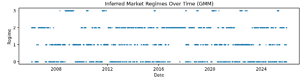
High-vol regime clusters around prolonged stress episodes, supporting interpretation as persistent market states.

Accuracy vs confidence, by regime

Figure 2

Out-of-sample accuracy versus confidence by regime

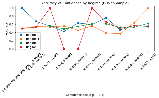
Confidence is not universally monotonic. High-vol regime shows degraded stability (and smaller bin counts).

Equity curve (OOS)

Figure 3

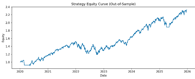
Selective deployment changes drawdowns/volatility more than it changes raw predictive metrics. Gross of costs.

Probability field + regimes

Figure 4

Logistic probability field with inferred regimes

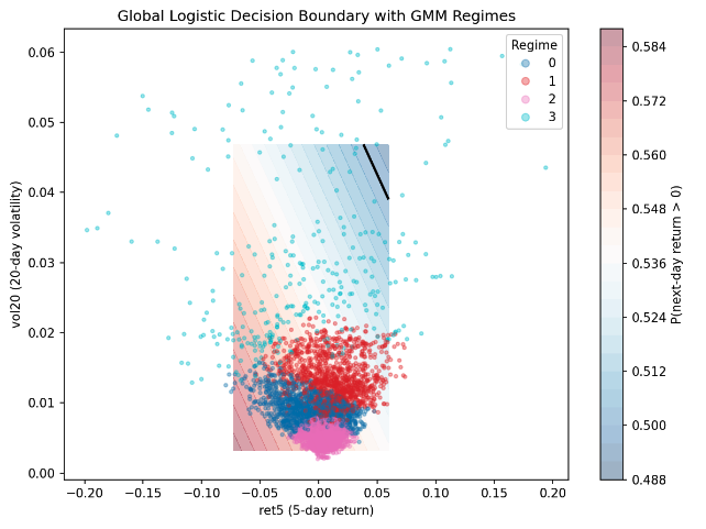
Regimes occupy distinct areas of (ret5, vol20), providing a geometric explanation for state-dependent behavior.

Probability compression

Figure 5

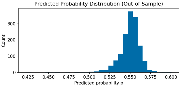
Predicted probabilities concentrate near the unconditional mean, motivating thresholded deployment.

Interpretation and limitations

Diagnostic, not “alpha claims.” The point is to map failure modes and decide when not to trade.
Costs not modeled. Results are gross of transaction costs, slippage, and financing/short constraints.
Small samples in extreme regimes. High-volatility regime bins can be thin; interpret bin-level spikes cautiously.
Next steps. Richer features, alternative regime definitions, and explicit execution costs would make the deployment test more realistic.