Key Numbers
Metrics are reported for model comparison and diagnostic clarity, not as a "forecast product" claim.
Executive Summary
- Prices are explained by standard hedonic structure controls, but residuals remain spatially structured.
- Distance-to-coast proxy (
lndist_pch) behaves like a location premium and becomes stronger under spatial correction. - Spatial dependence matters: ignoring it can distort magnitudes and confidence on key location terms.
- Cluster segmentation provides a clean way to encode micro-markets and stress-test heterogeneity.
Spatial Structure (Selected Visuals)
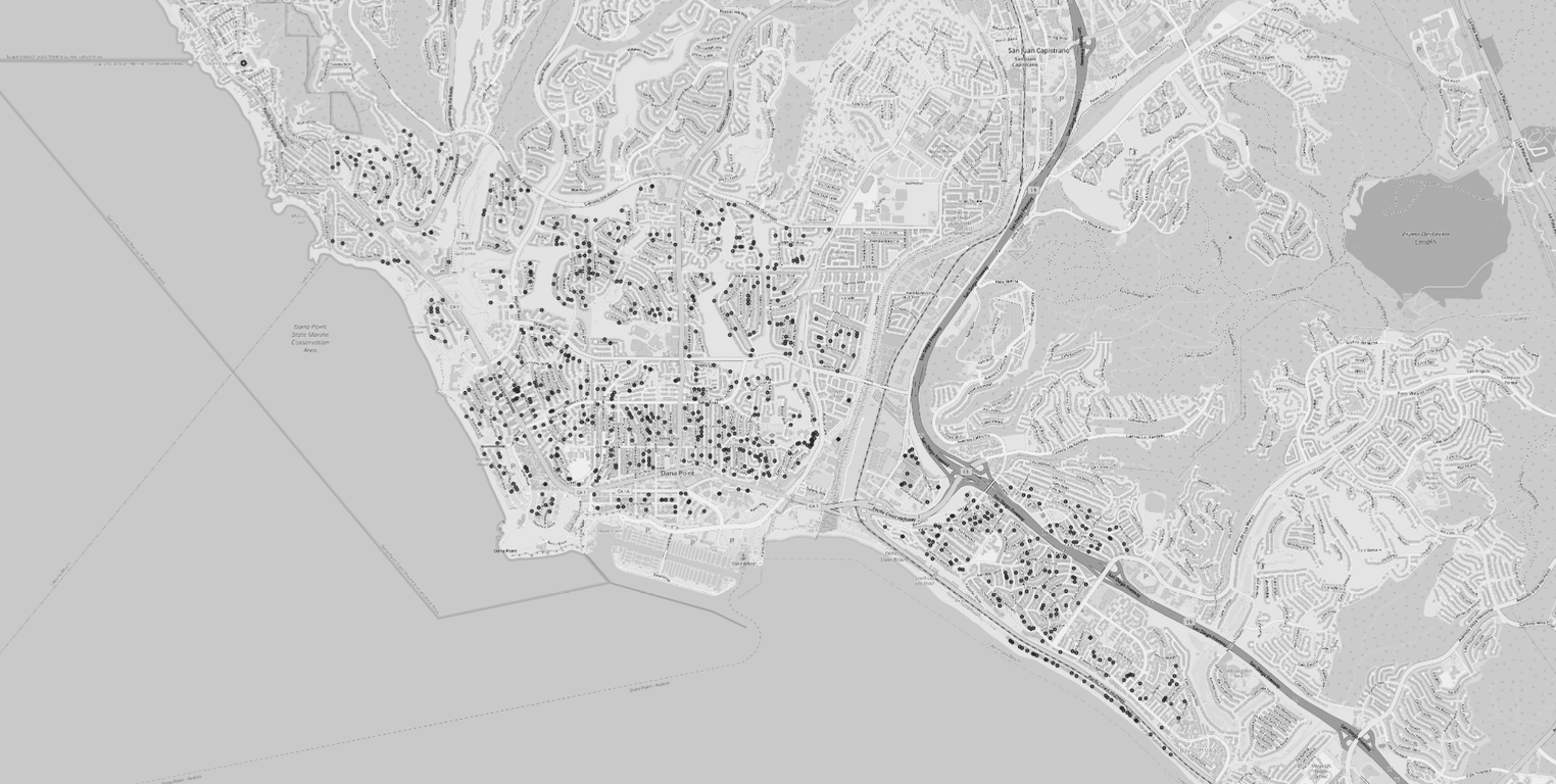
Used to validate spatial clustering and motivate spatial dependence correction.
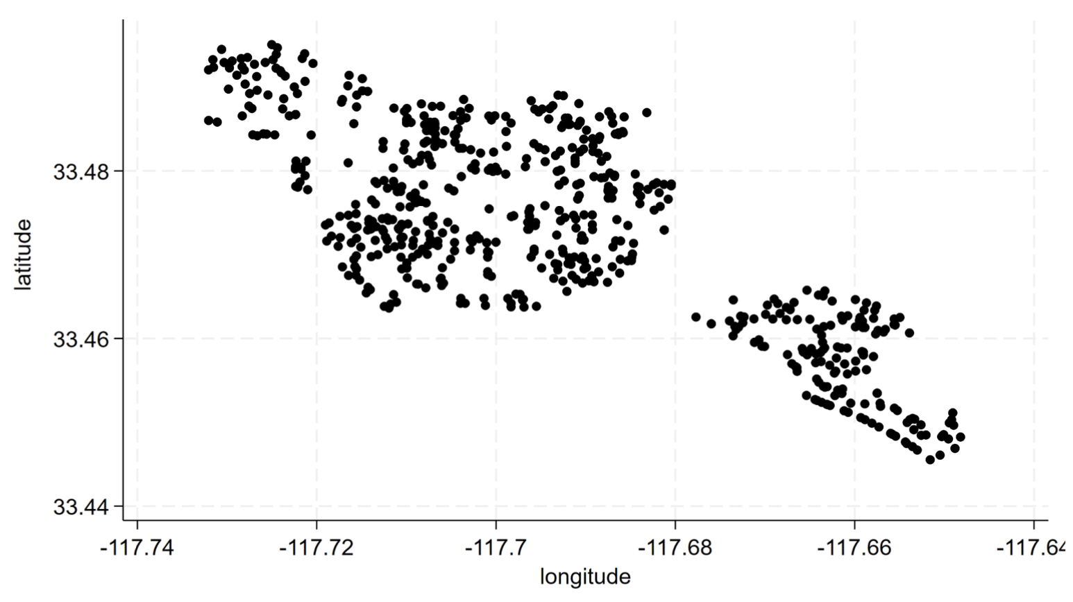
Spatial distribution of observations used to motivate spatial controls and segmentation.
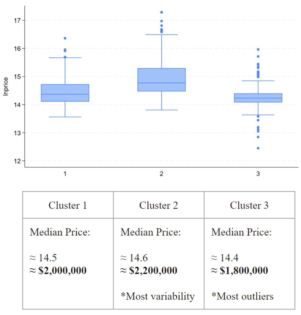
Cluster IDs are used as segmentation controls and for robustness checks.
Data Description (Descriptive Statistics)
Three control blocks are used: main structure controls, time controls, and spatial controls.
Main Controls
| Variable | Obs | Mean | Std. Dev. | Min | Max |
|---|---|---|---|---|---|
| house id | 620 | 310.5 | 179.123 | 1 | 620 |
| price | 620 | 2,875,487 | 3,175,359 | 380,000 | 32,000,000 |
| sqft | 620 | 2,554.19 | 1,391.42 | 799 | 13,777 |
| lot sqft | 620 | 8,877.55 | 21,439.87 | 1,000 | 304,920 |
| beds | 620 | 3.556 | 0.916 | 2 | 9 |
| baths | 620 | 2.585 | 1.151 | 1 | 10 |
| stories | 620 | 1.731 | 0.591 | 1 | 3 |
| parking | 620 | 2.25 | 0.689 | 1 | 8 |
| single family | 620 | 0.905 | 0.294 | 0 | 1 |
| condo | 620 | 0.044 | 0.204 | 0 | 1 |
| townhomes | 620 | 0.035 | 0.185 | 0 | 1 |
| duplex triplex | 620 | 0.016 | 0.126 | 0 | 1 |
| zipcode | 620 | 92627.74 | 2.171 | 92624 | 92629 |
| year built | 620 | 1980.78 | 16.465 | 1928 | 2023 |
| house by year | 620 | 627,925.91 | 362,230.01 | 2,022 | 1,254,260 |
Time Controls
| Variable | Obs | Mean | Std. Dev. | Min | Max |
|---|---|---|---|---|---|
| time | 620 | 753.721 | 10.194 | 739 | 772 |
| year=2021 | 620 | 0.232 | 0.423 | 0 | 1 |
| year=2022 | 620 | 0.318 | 0.466 | 0 | 1 |
| year=2023 | 620 | 0.335 | 0.473 | 0 | 1 |
| year=2024 | 620 | 0.115 | 0.319 | 0 | 1 |
| month dummies (1–12) | Included as indicator controls (means range ~0.053–0.113). | ||||
Spatial Controls
| Variable | Obs | Mean | Std. Dev. | Min | Max |
|---|---|---|---|---|---|
| dist_pch | 620 | 0.025 | 0.011 | 0.004 | 0.055 |
| latitude | 620 | 33.473 | 0.012 | 33.445 | 33.495 |
| longitude | 620 | -117.693 | 0.022 | -117.732 | -117.648 |
| kmeans cluster | 620 | 2.087 | 0.764 | 1 | 3 |
| std kmeans cluster | 620 | 1.979 | 0.724 | 1 | 3 |
| int complete cluster | 619 | 63.99 | 69.144 | 1 | 244 |
| int ward cluster | 619 | 135.008 | 123.454 | 1 | 393 |
Model 1: Spatial Autoregressive (GS2SLS / IV)
The goal is to estimate structural and location effects while correcting for spatial dependence and endogeneity. This specification is treated as the primary "pricing" model.
lnpricei = β0 + β1lnsqfti + β2bedsi + β3bathsi + β4lndist_pchi + β5storiesi + δ·Typei + i.month + i.year + εi
GS2SLS Estimates
| Term | Coef | Std. Err | z | P>z | 95% CI |
|---|---|---|---|---|---|
| lnsqft | 1.052 | 0.174 | 6.060 | 0.000 | [0.712, 1.392] |
| beds | -0.043 | 0.029 | -1.490 | 0.136 | [-0.101, 0.014] |
| baths | 0.091 | 0.033 | 2.800 | 0.005 | [0.027, 0.155] |
| lndist_pch | 0.424 | 0.039 | 10.780 | 0.000 | [0.347, 0.501] |
| stories | -0.134 | 0.036 | -3.680 | 0.000 | [-0.205, -0.062] |
| single_family | 0.112 | 0.050 | 2.220 | 0.026 | [0.013, 0.211] |
| year=2022 | 0.154 | 0.042 | 3.630 | 0.000 | [0.071, 0.237] |
| year=2023 | 0.199 | 0.040 | 4.920 | 0.000 | [0.120, 0.278] |
| year=2024 | 0.235 | 0.059 | 3.960 | 0.000 | [0.119, 0.352] |
| std_kmeans_cluster=2 | -0.337 | 0.036 | -9.440 | 0.000 | [-0.407, -0.267] |
| std_kmeans_cluster=3 | -0.277 | 0.036 | -7.660 | 0.000 | [-0.348, -0.206] |
| Constant | 8.079 | 1.225 | 6.590 | 0.000 | [5.678, 10.480] |
(1) Size dominates (lnsqft ≈ 1.05), consistent with multiplicative scaling of price with interior area. (2) Location premium is strong (lndist_pch positive and highly significant), especially clean under spatial correction. (3) Cluster effects are economically large, consistent with micro-market segmentation not captured by basic covariates.
Model 2: Logit Classifier (Price Regime / Tail Flag)
This model treats a price-state indicator as the target and tests whether structure + location + clusters reliably separate regimes. The purpose is diagnostic: "does the feature set actually separate outcomes cleanly?"
Pr(Di=1) = σ( β0 + β1sqfti + β2bedsi + β3bathsi + β4storiesi + β5single_familyi + β6dist_pchi + γ·ClusterIDi + i.month + i.year )
Logit Estimates
| Term | Coef | Std. Err | t | p | 95% CI | Sig |
|---|---|---|---|---|---|---|
| sqft | 0.002 | 0.000 | 7.61 | 0.000 | [0.001, 0.002] | *** |
| beds | -0.288 | 0.251 | -1.14 | 0.253 | [-0.780, 0.205] | |
| baths | 0.927 | 0.282 | 3.29 | 0.001 | [0.375, 1.479] | *** |
| stories | -1.295 | 0.361 | -3.58 | 0.000 | [-2.003, -0.587] | *** |
| single_family | 1.612 | 1.071 | 1.51 | 0.132 | [-0.487, 3.711] | |
| dist_pch | 61.788 | 20.044 | 3.08 | 0.002 | [22.502, 101.073] | *** |
| ClusterID=2 | 1.030 | 0.432 | 2.38 | 0.017 | [0.183, 1.878] | ** |
| ClusterID=3 | -0.611 | 0.500 | -1.22 | 0.222 | [-1.590, 0.369] | |
| Constant | -10.773 | 1.817 | -5.93 | 0.000 | [-14.334, -7.212] | *** |
(1) Size and bathrooms drive regime separation strongly. (2) dist_pch is economically meaningful in classification, not just in continuous pricing. (3) Clusters matter, consistent with submarket structure not fully reducible to raw coordinates.
Classification Diagnostics
| Metric | Value | Notes |
|---|---|---|
| Correctly classified | 90.48% | Threshold: Pr(D) ≥ 0.5 |
| Sensitivity | 74.84% | Pr(+ | D) |
| Specificity | 95.70% | Pr(- | ~D) |
| PPV | 85.29% | Pr(D | +) |
| NPV | 91.94% | Pr(~D | -) |
Diagnostics (Residual Structure)
Residual diagnostics are used to sanity-check fit, tail behavior, and whether structure-only modeling leaves spatial patterns behind.
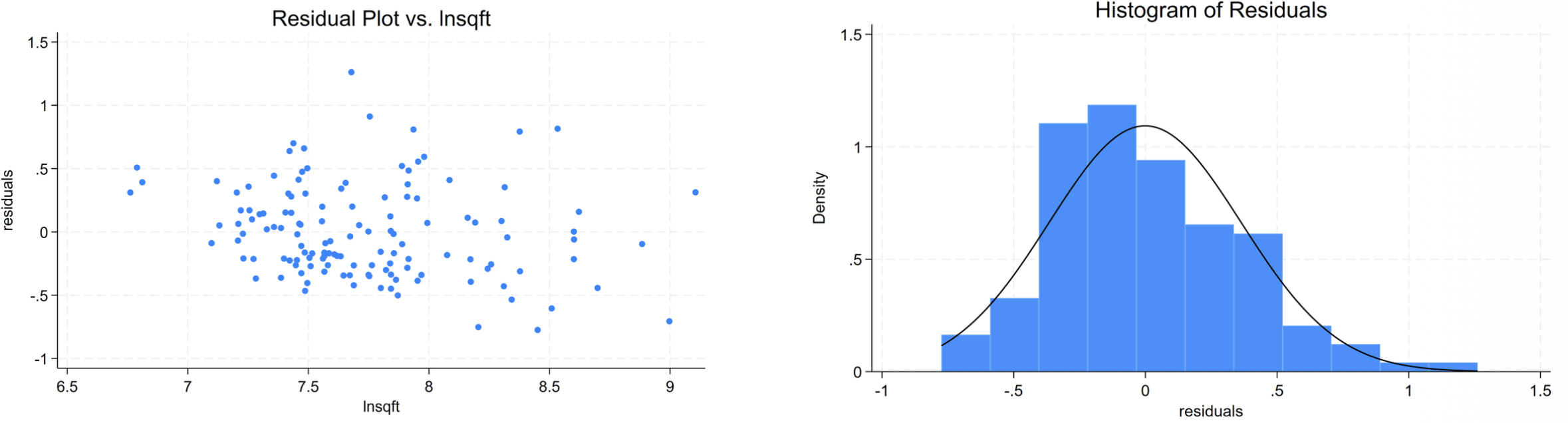
Used to check heteroskedasticity patterns and distributional shape (tails/skew).
Limitations & Next Steps
- Tail heaviness: The price distribution is extremely right-skewed, so robust checks matter.
- Micro-market stability: Cluster definitions can drift if the sample window expands or boundaries shift.
- Production upgrade path: Add richer geospatial features, nonlinear structure terms, and explicit spatial weight sensitivity tests.